How Do You Verify Microscope Image Comparability After Software Updates?

Verify microscope image comparability after a software update by testing two things separately: whether the same saved data produces equivalent results, and whether new acquisitions remain consistent with the previous workflow. Use representative archived images, stable reference specimens, matched settings, and acceptance limits tied to the measurements that matter. Images that look identical on screen can still differ in pixel values, spatial calibration, or object measurements.

Define comparability for the intended application before testing. Cell counting, fluorescence quantification, dimensional measurement, and qualitative morphology require different evidence. An update could preserve cell counts while changing measured fluorescence intensity, so a single pass-or-fail judgment for the entire microscope is rarely sufficient.

Where should the comparison start?

Preserve the existing workflow before installing the update, wherever possible. Record the application version, acquisition configuration, camera driver, relevant firmware, analysis settings, and export options. Keep representative original image files with their metadata. Screenshots and presentation exports cannot establish whether the underlying measurements have changed.

Build a baseline from repeated acquisitions and repeated analyses under the previous configuration. This establishes normal variability from illumination, focusing, specimen positioning, and analysis. A difference after updating becomes meaningful when compared with that baseline and the requirements of the assay.

If the update has already happened, use archived reference measurements, retained original files, and previous calibration records. Document the missing baseline explicitly. Without pre-update repeatability data, small differences are harder to attribute, and the evidence supports a narrower conclusion.

Separate software processing from image acquisition

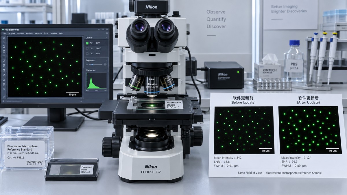
The most informative comparison uses two complementary tests. Reprocessing identical files isolates changes in import, processing, measurement, and export. Reimaging a stable specimen tests the acquisition workflow, including software-controlled hardware settings.

Confirm that “raw” files really contain unprocessed detector data. Some formats store corrected images or apply corrections during import. Preserve the earliest available data and identify which transformations occur before the file reaches the analysis stage.

When the old version remains available, use an isolated, supported installation for comparison. Keep the original files read-only and work on copies, especially if opening a project in the new version upgrades its format. Verify hardware compatibility before attempting acquisitions through an older installation.

Which reference specimens reveal useful differences?

A stage micrometer tests spatial calibration, but it does not establish fluorescence comparability. Fluorescent reference slides or suitable bead preparations reveal changes in signal, uniformity, and apparent feature size. A blank field or dark acquisition helps characterize background and detector offset. Select references that challenge the functions used in the actual workflow.

Include representative assay images spanning weak signals, dense objects, uneven backgrounds, and features close to the detection threshold. A bright, sparse specimen can pass while a dim biological image loses objects after a change in denoising or segmentation.

For physical specimens, record storage conditions, mounting medium, orientation, and time since preparation. Repeated fluorescence imaging introduces bleaching, while live specimens change during observation. Stable references and repeated baseline measurements provide a stronger comparison than a single biological field acquired twice.

Sample several fields and repeat acquisitions sufficiently to estimate variability. Different fields reveal illumination or positioning effects; repeated images of one field reveal short-term repeatability. Multiple pixels from the same image are not independent specimen replicates.

Matched settings require more than matching preset names

Inspect the saved acquisition parameters and the metadata of the resulting files. A preset with an unchanged name can inherit new defaults. For quantitative comparisons, disable automatic exposure, gain, contrast, and other adaptive controls unless they are part of the workflow being evaluated.

• Detector settings: exposure time, gain, binning, readout mode, bit depth, and region of interest affect recorded values and sampling.
• The objective, immersion medium, optical zoom, filters, and illumination configuration establish the optical comparison. Allow the instrument to reach its usual operating condition.
• For optical sections: preserve z-step spacing, pinhole settings where applicable, scan speed, averaging, and focus strategy. Equal projection images can conceal different stacks.
• Background correction, flat-field correction, deconvolution, denoising, and stitching need explicit settings. Record correction files and algorithm versions when available.

Matching a laser-power percentage or lamp setting does not prove equal illumination at the specimen. Source output and control behavior can change. Use reference intensity measurements or an appropriate illumination measurement when intensity comparability matters.

Keep focus and image registration under control. Small axial shifts change brightness and apparent sharpness, particularly in optical-sectioning workflows. Registration helps compare corresponding structures, but interpolation changes pixel values. Evaluate original images for intensity measurements and document any registration used for spatial comparisons.

Which measurements should agree?

Choose metrics that connect directly to the reported result. Assess spatial calibration using a reference with known dimensions: verify both axes, reported units, and relevant z-spacing. A metadata error can preserve the visible image while changing every reported area or volume.

For intensity measurements, compare background, background-corrected signal, signal distribution, and the fraction of saturated pixels. Use the same regions and calculation rules. A similar average intensity can hide clipping of bright structures or loss of weak features.

Noise needs its own assessment. Repeated dark or uniform-field acquisitions help distinguish detector variation from spatial specimen structure. Denoising can lower apparent noise while altering texture, small objects, and subsequent measurements. A cleaner-looking image is not sufficient evidence of equivalence.

Assess resolution and feature appearance using suitable reference structures. Bead profiles can reveal changes in apparent width, but their interpretation depends on bead size, focus, optical conditions, and sampling. They are most useful as controlled comparisons within the same configuration.

For multichannel imaging, inspect channel identity and spatial alignment. A change in channel ordering or registration can alter colocalization results even when each individual channel appears acceptable.

Finally, compare the actual outputs: object count, area, length, integrated intensity, classification, or another assay endpoint. Review the overlays alongside the numbers. An unchanged count can conceal different detected objects, split boundaries, or merged neighbors.

How much difference is acceptable?

Set acceptance limits before examining the update results. Base them on baseline repeatability, measurement uncertainty, and the smallest difference that would affect interpretation. There is no universal percentage tolerance that establishes comparability across microscopy applications.

Use paired comparisons when the same files, fields, or objects are available. Inspect the difference between versions and whether that difference grows with signal level, object size, or position in the image. A proportional intensity change requires a different response from a constant background offset.

A correlation coefficient alone is insufficient. Measurements can correlate closely while one version consistently reports larger values. Likewise, a statistically nonsignificant difference does not demonstrate equivalence. Assess whether the estimated bias and its uncertainty fall within the predefined acceptable range, using enough independent observations to support that judgment.

Percentage differences become unstable near zero. For low-background signals or very small objects, use absolute differences or an assay-relevant scale. Separate results by relevant conditions when a pooled average would conceal failures, such as agreement for bright objects alongside disagreement for dim ones.

Why do images look the same when measurements change?

Display scaling often masks numerical differences. Independently applied lookup tables can make two images look equally bright even when their pixel values differ. Compare them using identical display limits, then examine the underlying data. Conversely, a new default display range can make unchanged data appear different.

File interpretation is another source of hidden changes. Inspect pixel dimensions, physical pixel size, units, channel labels, timestamps, z-spacing, and bit depth after import and export. Confirm that an unsigned intensity range has not been rescaled or converted during transfer.

Lossy compression, reduced-bit-depth exports, and baked-in contrast adjustments can compromise quantitative comparisons. Test the actual export-and-import route used downstream. If acquisition and analysis occur in different applications, a correct acquisition file does not guarantee that its calibration survives the transfer.

Changed segmentation defaults deserve particular attention. Threshold rules, edge handling, minimum object size, and treatment of touching objects can shift results without an obvious change in the displayed image. Inspect difficult examples directly rather than relying only on aggregate measurements.

What should happen when the comparison fails?

Locate the first stage where results diverge. If identical archived files change on import, investigate decoding and metadata interpretation. If imported pixels agree but masks differ, examine processing and segmentation. If masks agree but measurements differ, investigate calibration and measurement definitions.

When archived-data analysis agrees but new acquisitions differ, examine hardware control, focus, illumination, detector settings, and correction files. Repeat the reference acquisition after resolving the suspected cause. Change one relevant setting at a time so the retest explains the discrepancy.

For longitudinal datasets, preserve acquisition and analysis version information. Reprocessing all retained raw images through one validated pipeline can resolve an analysis-version difference, provided the files contain sufficient information. It cannot repair saturation, missing channels, or acquisition settings that changed the recorded signal.

A correction factor requires evidence across the relevant measurement range and specimens. A relationship observed on one bright reference slide is insufficient for adjusting weak cellular signals or complex segmentation outputs.

What record supports a comparability decision?

Retain the reference files, configuration records, calibration results, analysis outputs, and representative overlays together. State the workflows tested, acceptance limits, observed differences, unresolved issues, and final decision. Include the full route from acquisition through exported measurements.

Describe the conclusion at the level supported by the evidence: for example, spatial measurements agree under the tested configuration, while fluorescence quantification remains unresolved. Reuse that verified configuration for subsequent work, and reassess when a later change affects the acquisition or analysis functions on which the conclusion depends.